1. Project Background

This report summarizes the visualization component of the research project “Examining Community College Student Enrollment and Completions in Green Sector Occupations”, a joint effort by the Community College Research Center (CCRC) and the University of Tennessee, Knoxville. My role was to design and implement an interactive visualization tool that shows how community college green program completions (“supply”) align with green-sector job postings (“demand”).

Community colleges need to align their training programs with the rapidly growing green economy, while also ensuring equitable access. However, a nationwide, interactive visualization of this alignment is currently lacking. Our project addresses this gap by:

Supply: Tracking completions in green programs from IPEDS (2012–2022).
Demand: Mapping green job postings from Lightcast (2010–2024), aggregated by Commuting Zone (CZ).
Classification: Applying O*NET “Greening of Work” categories.

2. Data Sources

2.1 IPEDS Supply Data

File: ccrc_cip_comp.dta
Key Fields: unitid, instnm, latitude, longitude, year, greencat, cmplt_tot

2.2 Lightcast Demand Data

File: lightcast-soc-year-county.csv
Fields: COUNTY (FIPS), YEAR, SOC_CODE, JOB_POSTING_COUNT, GREEN flag

2.3 Spatial Data

County Boundaries: county20/county20.shp
Commuting Zone Boundaries: cz20/cz20.shp
Mask Polygon: mask_polygon.geojson (generated via prepare_mask_polygon.R)

3. Data Preparation

3.1 Supply‐Side Wrangling

library(haven)
library(dplyr)

ccrc_cip_comp <- read_dta("ccrc_cip_comp.dta") %>%
  mutate(year = as.numeric(year))

saveRDS(ccrc_cip_comp, "ccrc_cip_comp.rds")

3.2 Demand‐Side Wrangling

library(sf)
library(readr)
library(dplyr)

# Read commuting zone geometries
CZ2020 <- st_read("cz20/cz20.shp") %>% select(CZ20 = cz, geometry)

# Read and filter Lightcast data
cz_raw <- read_csv("lightcast-soc-year-county.csv") %>%
  filter(GREEN == 1) %>%
  rename(YEAR = YEAR, green_job_postings = JOB_POSTING_COUNT)

# Merge and simplify
gz_sf <- cz_raw %>%
  inner_join(CZ2020, by = "CZ20") %>%
  st_as_sf() %>%
  st_transform(4326) %>%
  st_simplify(dTolerance = 0.05)
gz_sf$id <- seq_len(nrow(gz_sf))

saveRDS(gz_sf, "CZ_job_post.rds")

3.3 Mask Polygon Generation

library(rnaturalearth)
library(sf)
library(geojsonio)

us_states <- ne_states(country = "United States of America", returnclass = "sf")
us_poly   <- st_union(us_states) %>% st_transform(4326)

world_poly <- st_sfc(
  st_polygon(list(matrix(
    c(-180,-90, 180,-90, 180,90, -180,90, -180,-90),
    ncol = 2, byrow = TRUE
  ))),
  crs = 4326
)

mask_poly <- st_difference(world_poly, us_poly)
geojson_write(mask_poly, file = "mask_polygon.geojson")

3.4 JSON Export for Front-end

library(geojsonio)
library(dplyr)

# Export CZ GeoJSON per year
cz_df <- readRDS("CZ_job_post.rds")
for (yr in unique(cz_df$YEAR)) {
  geojson_write(
    filter(cz_df, YEAR == yr),
    file = sprintf("CZData_%d.json", yr)
  )
}

# Export institution GeoJSON per year
inst_df <- readRDS("ccrc_cip_comp.rds") %>%
  filter(!is.na(longitude), !is.na(latitude)) %>%
  st_as_sf(coords = c("longitude", "latitude"), crs = 4326) %>%
  select(year, instnm, inst_perc_green_tot)

for (yr in unique(inst_df$year)) {
  geojson_write(
    filter(inst_df, year == yr),
    file = sprintf("InstituteData_%d.json", yr)
  )
}

3.5 Analytic Pipeline & Preparation

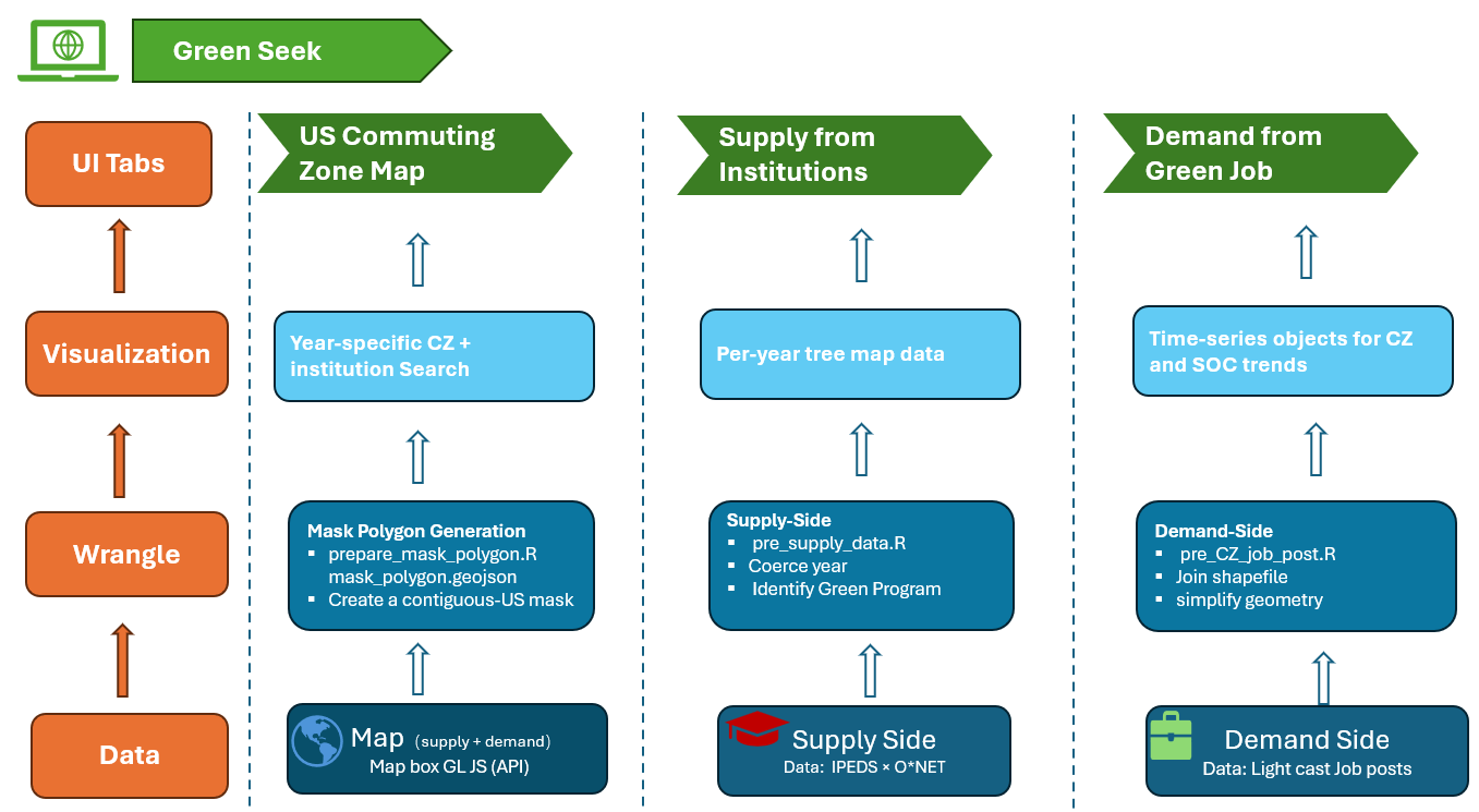
The analytic pipeline consists of several R scripts that perform data wrangling, JSON export, and visualization preparation. The key components are: - Supply-Side Wrangling: pre_supply_data.R reads ccrc_cip_comp.dta, coerces year to numeric, sorts institution names, and writes ccrc_cip_comp.rds for downstream use. - Demand-Side Wrangling: pre_CZ_job_post.R loads Lightcast CSVs (filtered GREEN == 1 for 2010–2023), aggregates postings by county/SOC, joins to county20 and CZ2020 shapefiles, simplifies geometries (dTolerance = 0.05), and saves CZ_job_post.rds. - Mask Polygon Generation: prepare_mask_polygon.R fetches U.S. state boundaries via rnaturalearth, unions them, computes the geometric difference from a world polygon to mask out non-contiguous areas, and exports mask_polygon.geojson. - GeoJSON Exports for Front-end: pre_cz jason.R writes per-year CZ GeoJSON files (CZData_<year>.json) from CZ_job_post.rds. Pre_supply_json.R converts ccrc_cip_comp.rds into point SF, selects instnm and inst_perc_green_tot, and exports InstituteData_<year>.json for each year. - Visualization Preprocessing: Pre_treemap.R aggregates green completions by program title, builds a per-year Plotly treemap list (Green_degree_treemap_plotly_list.rds). Pre_Plotly.R computes time-series of green job proportions by CZ and by SOC, converts ggplots to Plotly objects, and writes p_CZ_plotly.rds & p_SOC_plotly.rds.

4. Interactive Application

4.1 Shiny UI & Server

library(shiny)
library(jsonlite)
library(geojsonio)
library(dplyr)
library(sf)
library(plotly)

source("mapboxtoken_setup.R")
ccrc_data <- readRDS("ccrc_cip_comp.rds")
cz_data   <- readRDS("CZ_job_post.rds") %>% mutate(id = row_number())

ui <- fluidPage(
  titlePanel("CCRC Green Seek"),
  fluidRow(
    column(4,
      selectInput("selected_year", "Year", choices = sort(unique(cz_data$YEAR))),
      plotlyOutput("treemapPlot")
    ),
    column(8,
      selectizeInput("search_term", "Search Institution", choices = NULL),
      actionButton("search_btn", "Search"),
      tags$button("Clear", onclick = "clearMap()"),
      div(id = "map", style = "height:600px;")
    )
  ),
  fluidRow(
    column(6, plotlyOutput("cz_plot")),
    column(6, plotlyOutput("trendPlot"))
  )
)

server <- function(input, output, session) {
  observe({
    req(input$selected_year)
    insts <- ccrc_data %>%
      filter(year == input$selected_year) %>%
      pull(instnm) %>%
      unique() %>%
      sort()
    updateSelectizeInput(session, "search_term", choices = insts, server = TRUE)
    session$sendCustomMessage("loadYear", input$selected_year)
    session$sendCustomMessage("loadInstituteYear", input$selected_year)
  })
  observeEvent(input$search_btn, {
    res <- ccrc_data %>%
      filter(instnm == input$search_term, year == input$selected_year) %>%
      slice(1)
    if (nrow(res)) {
      popup <- paste0("<strong>", res$instnm, "</strong><br>Green %: ",
        sprintf("%.1f%%", res$inst_perc_green_tot * 100))
      session$sendCustomMessage("updateSearch", list(
        lng = res$longitude, lat = res$latitude, popup = popup
      ))
    }
  })
  output$treemapPlot <- renderPlotly({
    readRDS("Green_degree_treemap_plotly_list.rds")[[as.character(input$selected_year)]]
  })
  output$cz_plot    <- renderPlotly(readRDS("p_CZ_plotly.rds"))
  output$trendPlot  <- renderPlotly(readRDS("p_SOC_plotly.rds"))
}

shinyApp(ui, server)

4.2 Mapbox Front-end (mapbox.js)

mapboxgl.accessToken = mapboxToken;
const map = new mapboxgl.Map({
  container: 'map',
  style: 'mapbox://styles/mapbox/navigation-day-v1',
  center: [-95, 40],
  zoom: 3.5
});

function loadCZData(year) {
  fetch(`CZData_${year}.json`)
    .then(res => res.json())
    .then(data => {
      if (map.getSource('cz')) {
        map.getSource('cz').setData(data);
      } else {
        map.addSource('cz', { type: 'geojson', data });
        map.addLayer({
          id: 'cz-layer',
          type: 'fill',
          source: 'cz',
          paint: { /* color & opacity settings */ }
        });
      }
    });
}

function loadInstituteData(year) {
  fetch(`InstituteData_${year}.json`)
    .then(res => res.json())
    .then(data => {
      if (!map.getSource('institutes')) {
        map.addSource('institutes', { type: 'geojson', data });
        map.addLayer({
          id: 'institutes-layer',
          type: 'circle',
          source: 'institutes',
          paint: {
            'circle-radius': [
              'interpolate', ['linear'], ['get', 'inst_perc_green_tot'],
              0, 4, 1, 12
            ]
          }
        });
      } else {
        map.getSource('institutes').setData(data);
      }
    });
}

Shiny.addCustomMessageHandler('loadYear', loadCZData);
Shiny.addCustomMessageHandler('loadInstituteYear', loadInstituteData);
Shiny.addCustomMessageHandler('updateSearch', coords => {
  map.flyTo({ center: [coords.lng, coords.lat], zoom: 6 });
  new mapboxgl.Popup()
    .setLngLat([coords.lng, coords.lat])
    .setHTML(coords.popup)
    .addTo(map);
});

map.on('mousemove', 'cz-layer', e => { /* hover effect */ });
map.on('mouseleave', 'cz-layer', () => { /* remove hover */ });
window.clearMap = () => map.flyTo({ center: [-95, 40], zoom: 3.5 });

5. APP UI Key Features

6. Conclusions & Next Steps

The interactive map and time-series charts reveal spatial disparities in green job demand and highlight regions where community colleges may need to expand their green programs.
Future enhancements include demographic filters (race, gender), predictive modeling, and user-uploaded data integration.

6.1 Future Extensions & Reusability

This R preprocessing + Mapbox GL JS pipeline can ingest new supply/demand datasets by replacing JSON export scripts. Future enhancements may include demographic filtering, predictive analytics tabs, and user data uploads, building on the existing Shiny + Mapbox framework.

7. Repository

Full code and documentation available at:

GitHub · wwang93/CCRC_GreenSeek-Mapping

8 Full Paper

For comprehensive analysis, methodology, and further implications:

Access the Full Paper (Google Doc)

CCRC Green Seek: Mapping Community College Green Sector Alignment